Code to reproduce Figure 5 from doi: 10.1172/jci.insight.121899

Raw data is here: BioProject ID: PRJNA445968

Figure 5

setwd("~/Desktop/Charles_MAIT/") #pick a directory
rm(list=ls())
library(plyr);library(ggtree);library(phyloseq);library(ggplot2);library(scales);library(grid)
library(Hmisc);library(gridExtra);library(scales);library(stringr);library(logistf)
library(coxphf);library(reshape2);library(ifultools);library(car);library(vegan)
library(gdata);library(chron);library(data.table);library(tidyr) #imports tibble
library(ggplot2);library(yingtools2);library(gridExtra);library(lubridate);library(dplyr)
library("pheatmap");library("RColorBrewer");library("genefilter");library(ggthemes)
library("reshape2");library("gridExtra");library("colorspace");library("lattice")
library("pracma");library("ComplexHeatmap");library("BiocParallel");library("viridis");library("circlize")
select <- dplyr::select
summarize <- dplyr::summarize
rownames_to_column <- tibble::rownames_to_column

phy_contacts <- readRDS("phy.JCI.RDS") #this is in the uparse folder on GitHub

Clinical variables

# Calculate bray curtis distance matrix
bray <- phyloseq::distance(phy_contacts, method = "bray")

# make a data frame from the sample_data
sampledf <- data.frame(sample_data(phy_contacts))

# Adonis test
library(vegan)
set.seed(12345678)
adonis2(bray ~ IGRA + sex + Group6_TB_category, data = sampledf)

Permutation test for adonis under reduced model Terms added sequentially (first to last) Permutation: free Number of permutations: 999

	Df	SumsOfSqs	MeanSqs	F.Model	R2	Pr(>F)
IGRA	1	0.03927	0.01281	0.6705	0.851
sex	2	0.17300	0.05644	1.4769	0.072	.
Group6_TB_category	1	0.21748	0.07095	3.7132	0.001	***
Residual	45	2.63568 0.85981
Total	49	3.06544	1.00000
---

This indicates that the variable 'Group6_TB_category' explains the variation between individuals given their microbiome compositioin (***), but IGRA status and sex do not contribute to this variation.

beta <- betadisper(bray, sampledf$Group6_TB_category)
permutest(beta)

Permutation test for homogeneity of multivariate dispersions Permutation: free Number of permutations: 999

	Df	Sum Sq	Mean Sq	F	N.Perm	Pr(>F)
Groups	1	0.00044	0.00044028	0.1967	999	0.663
Residuals	48	0.10747	0.00223889

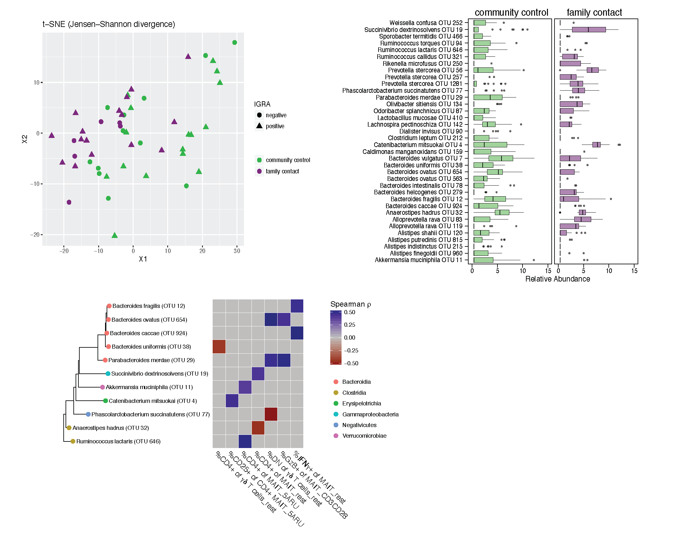
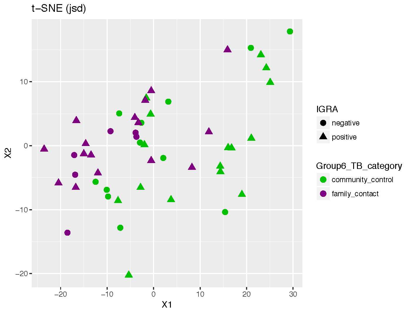
Determining microbiome differences

#tsne plots
library(phyloseq)
library(tsnemicrobiota)
library(ggplot2)

tsne_res <- tsne_phyloseq(phy_contacts, distance='jsd',perplexity = 8, verbose=0, rng_seed = 3901,dimensions=3)

# Plot the results.
#sample_data(phy_contacts)$cd4m_5aru <- as.numeric(as.character(sample_data(phy_contacts)$cd4m_5aru))

plot_tsne_phyloseq(phy_contacts, tsne_res,
  color = 'Group6_TB_category',shape="IGRA", title='t-SNE (jsd)') +
  geom_point(size=3) + scale_color_manual(values=c(Palette_FC_CC))+
  scale_fill_manual(values=c(Palette_FC_CC))

#docker run -v ~/Desktop/Charles_MAIT/:/home/linuxbrew/inputs -it biobakery/lefse bash

N.B. Running LEfSe locally can be difficult if your system("echo $PATH") within R doesn't contain the LEfSe scripts, or if you constantly update R packages (like I do). This is guarenteed to cause problems with running LEfSe (e.g., rpy2 doesn't seem to be supported on my Mac any longer), so I've found docker to be an easy option. I run the above command on the command line, and can then run subsequent commands from R.

system("echo $PATH")
results_folder <- "~/Desktop/Charles_MAIT/" 

#make names lefse-friendly for python scripts
taxa_names(phy_contacts)<-gsub('\\(','',taxa_names(phy_contacts))
taxa_names(phy_contacts)<-gsub(')','',taxa_names(phy_contacts))
taxa_names(phy_contacts)<-gsub(' ','_',taxa_names(phy_contacts))
taxa_names(phy_contacts)
phy.lefse<-phy_contacts

class <- "Group6_TB_category"
subclass<-NA
subject<-"sample"
anova.alpha<-0.01
wilcoxon.alpha<-0.01
lda.cutoff<-2.5

wilcoxon.within.subclass <- TRUE
one.against.one <- FALSE 
mult.test.correction <- 0 
make.lefse.plots <- FALSE
by_otus <- FALSE
# 
sample.data <- phyloseq::sample_data(phy.lefse) %>% data.frame(stringsAsFactors = FALSE)
sample.data <- rownames_to_column(sample.data,var="sample") 
# 
keepvars <- c("sample","Group6_TB_category")
keepvars <- unique(keepvars[!is.na(keepvars)])

lefse.samp <- sample.data[, keepvars]
# 
sample0 <- t(lefse.samp) %>% as.matrix()
colnames(sample0) <- sample0[1,]
sample0 <- as.data.frame(sample0) %>% t() %>% as.data.frame()

data0 <- otu_table(phy.lefse) %>% as.data.frame()
data1 <- data0 %>% as.data.table(keep.rownames=T) %>% t()
data2 <- rownames_to_column(as.data.frame(data1),var="sample")

pre.lefse <- right_join(sample0,data2,by="sample") %>% t()
rownames(pre.lefse) <- NULL
pre.lefse[1,1] <- "sample"
pre.lefse[2,1] <- "IGRA"
pre.lefse <- pre.lefse %>% t() %>% na.omit() %>% t()
# 

write.table(pre.lefse,file =paste(results_folder,"lefse.txt",sep=""),sep = "\t",row.names = FALSE,col.names = FALSE,quote = FALSE)
# 
opt.class <- paste("-c", which(keepvars %in% class))
opt.subclass <- ifelse(is.na(subclass), "", paste("-s", which(keepvars %in% subclass)))
opt.subject <- ifelse(is.na(subject), "", paste("-u", which(keepvars %in% subject)))
format.command <- paste(paste("format_input.py ",results_folder,"lefse.txt ",results_folder,"lefse.in",sep=""), opt.class, opt.subclass, opt.subject, "-o 1000000")
system(format.command)
#
#docker run -v ~/Desktop/Charles_MAIT/:/home/linuxbrew/inputs -it biobakery/lefse bash
lefse.command <- paste(paste("run_lefse.py ","lefse.in " , "lefse.res",sep=""), 
                       "-a", anova.alpha, "-w", wilcoxon.alpha, "-l", lda.cutoff, 
                       "-e", as.numeric(wilcoxon.within.subclass), "-y", as.numeric(one.against.one), 
                       "-s", mult.test.correction)
lefse.command
system(lefse.command)

lefse.out <- read.table(paste("lefse.res",sep=""), header = FALSE, sep = "\t")
names(lefse.out)<-c("taxon","log.max.pct","direction","lda","p.value")
(lefse.out<-na.omit(lefse.out))
Palette_LTBI_treatment <- c("#377eb8","#984ea3") #modify this

ltk<-as.character(lefse.out$taxon)
phy_ra_ltk<-prune_taxa(ltk,phy_contacts)
phy_ra_ltk_m<-psmelt(phy_ra_ltk)

Palette_FC_CC <- c("#00C000","#7F007F")
g2<-ggplot(phy_ra_ltk_m,aes(x=OTU,
  y=Abundance,color=Group6_TB_category,
  fill=Group6_TB_category))+
  geom_boxplot(position=position_dodge(),
   colour="black", # Use black outlines,
    size=.3,alpha=0.5) +      # Thinner lines
  theme_base()+
  xlab("")+
  coord_flip()+ facet_wrap(~Group6_TB_category) + 
  scale_y_continuous(limits = c(0,15))
if(length(unique(lefse.out$direction))<3){
  g2<-g2+scale_color_manual(values=c(Palette_FC_CC))+
    scale_fill_manual(values=c(Palette_FC_CC))
}
print(g2)

![abundance_plot](img/MAIT_GD/Correlated_FC-CC_0.01_LDA2.5_all.png)

Determining immune phenotype differences

This for loop correlated specifc immune phenotypes (vars_to_keep) with microbiota abundance. It generates a lot of intermediate plots of the individual correlations, but I won't show those.

#big for loop
mainDir <- "~/Desktop/Charles_MAIT/"
subDir <- "DESeq_FC-CC_immune"
dir.create(file.path(mainDir, subDir), showWarnings = TRUE,recursive = TRUE)
results_folder <- paste(mainDir,subDir,sep="")

cor_ht_dt <- NULL
heat_dt <- data.frame(taxon = NULL, rho = NULL, effectors = NULL)

sample_variables(phy)

vars_to_keep <- c("cd4gdpctcd4t","cd4gd","dngd","cd4mpctm_rest","cd4mpctm_5aru","cd8mpctm_rest","cd8mpctm_5aru",
"cd8mpctcd8t_5aru","dnmpctm_rest","cd8mcd69_5aru_minus_rest", "cd4mcd25_rest","cd4mcd25_5aru","cd8mcd25_rest","cd8mcd25_5aru","cd8mcd25_5aru_minus_rest", "gzbm_dyna","gzbm_rest","gzbm_dyna_rest","ifngm_dyna","ifngm_rest","ifng_dyna_rest") 

effectors_all<- c(vars_to_keep) 

for (effectors in effectors_all){
  # Subset the samples 
  phy_var <- subset_samples(phy_contacts,!is.na(get_variable(phy_contacts, effectors)) | get_variable(phy_contacts, effectors)!="")
  phy_var <-  subset_samples(phy_var, get_variable(phy_var, effectors) != "na")
  phy_var <-  subset_samples(phy_var, get_variable(phy_var, effectors) != "")

  sdat<-otu_table(phy_var) %>% as.data.frame()
  xcor<-get_variable(phy_var, effectors)
  c_th<-0.05
  c_pvalue<-list()
  c_estimate<-list()
  for (ic in seq(1,nrow(sdat))){
    ycor<-sdat[ic,]
    cor.result<-cor.test(as.numeric(xcor),as.numeric(ycor),method = "spearman") #nonparametric = spearman
    c_pvalue[[ic]] <- cor.result$p.value
    c_estimate[[ic]] <- cor.result$estimate
  }
  c_pvalue<-do.call('rbind',c_pvalue)
  c_estimate<-do.call('rbind',c_estimate)

  isig<-which(c_pvalue <= c_th)
  taxa_sig<-taxa_names(phy_var)[isig]
  c_pvalue_sig<-c_pvalue[isig]
  c_estimate_sig<-c_estimate[isig]
  correlation_results<-data.frame(taxa_sig,c_pvalue_sig,c_estimate_sig)
  names(correlation_results)<-c("taxon","pvalue","spearman_rho")

  if(nrow(correlation_results) > 0){

    correlation_results$rho<-as.numeric(correlation_results$spearman_rho)
    correlation_results$taxon<-factor(correlation_results$taxon,
                                      levels=correlation_results$taxon[order(correlation_results$spearman_rho)])
    correlation_results$i_eff <- effectors  

    # Cut off for rho    0.4 <= spearman_rho & spearman_rho  <=  -0.4
    correlation_results <- correlation_results[which(abs(correlation_results$spearman_rho) >= 0.2) ,]

    if(nrow(correlation_results) > 0){

      cor_ht_dt <- rbind(cor_ht_dt, correlation_results)  

      # barplot
      pdf(paste(results_folder,paste0("bar_plot_spearman_coeff",effectors,".pdf"),sep="/"),height = 6, width = 10)
      g1<-ggplot(data=correlation_results,aes(x=taxon, y=rho))+
        geom_bar(stat="identity")+ 
        coord_flip()+
        theme_base()+
        xlab("Species")+
        ylab("Spearman - rho")
      print(g1)
      dev.off()

      # code below is for heatmap

      phy_sig_var <-  prune_taxa(as.character(correlation_results$taxon), phy_var)
      sig_data_c<-data.frame(otu_table(phy_sig_var))
      y_eff <- as.numeric(as.character(get_variable(phy_sig_var, effectors)))



      pnca_colors<-colorRamp2(c(min(log(y_eff+1)),
                                max(log(y_eff+1))), c("white", "blue"))

      dist_to_use<-function(x) (1-dist(t(x)))
      mat<-as.matrix(as.data.frame(sig_data_c))     
      mat2<-scale(t(mat), scale = T, center = T)
      mat2<-t(mat2)
      annotations<-data.frame(y_eff,as.character(get_variable(phy_var, "Group6_TB_category")))
      names(annotations)<-c("effectors","group")

      tmp_c <- sample_data(phy_var) %>% as.data.frame()
      #tmp_c[order(tmp_c)$effectors,] #[order(sample_data(phy_var)$effectors),]

      max_value <- max(as.numeric(as.character(get_variable(phy_var, effectors))))
      #color_col = list(effectors = colorRamp2(c(0,max_value),c("white","#DC143C")), 
                                          #group = c("family_contact" = "#7F007F","community_control" = "#00C000"))

      #color_col = list(effectors = colorRamp2(c(0,noquote(max(tmp_c$effectors))),c("white","#DC143C")), group = c("family_contact" =   "#7F007F","community_control" = "#00C000"))
      #ha_column = HeatmapAnnotation(annotations, col = color_col)
      ha_column = HeatmapAnnotation(annotations)

      ht1 = Heatmap(mat2, name = "Relative Abundance", column_title = NA, top_annotation = ha_column,
                    clustering_distance_rows = "euclidean",
                    clustering_method_rows = "complete",row_names_side = "left", km=1, color_space = "LAB",
                    col=viridis(11), row_dend_side="right",
                    clustering_method_columns = "ward.D",
                    width=4, row_names_max_width = unit(8, "cm"),show_column_names= F,
                    row_names_gp = gpar(fontsize = 9), cluster_columns = T,na_col="white")
      ht_list = ht1
      padding = unit.c(unit(2, "mm"), grobWidth(textGrob("jnbksdffsdfsfd_annotation_name")) - unit(1, "cm"),
                       unit(c(2, 2), "mm"))


      pdf(paste(results_folder,paste0("heatmap_spearman_0.01_",effectors,".pdf"),sep="/"),height = 2.5, width = 11)
      draw(ht_list, padding = padding)
      dev.off()

    }
  }
}

# Reshape the dataframe for heatmap
cor_ht_dt <-  cor_ht_dt[,c("taxon","rho","i_eff")]

# Convert long to wide format for phyloseq object
cor_ht_dt_w <- dcast(cor_ht_dt, taxon ~ i_eff, value.var="rho",fun.aggregate = mean)
cor_ht_dt_w[is.na(cor_ht_dt_w)] <- 0

######match tree with heatmap rownames
phy_sig<-prune_taxa(as.character(cor_ht_dt_w$taxon),phy_contacts)

row_den <-  ape:::as.phylo(phy_tree(phy_sig))
# row_den <- as.dendrogram(hclust(dist(cor_data)))
# plot(row_den)

#r_order <-  rev(row_den$tip.label)
cor_data  <- cor_ht_dt_w
rownames(cor_data) <- cor_data$taxon
cor_data$taxon <- NULL

clust.col <- hclust(dist(t(cor_data)))
plot(clust.col)
col_den <- as.dendrogram(clust.col)
sig_data_c <- cor_data
mat<-as.matrix(sig_data_c)
mat2<-scale(t(mat), scale = F, center = F)
mat2<-t(mat2)
#rownames(mat2) <-  cor_ht_dt_w$taxon

# #get data from ggTree
# d <- fortify(tr)
# dd <- subset(d, isTip)
# r_order <- dd$label[order(dd$y, decreasing=T)]
# 
# mat3 <- mat2[match(r_order,rownames(mat2)),]

# Without phylogenetic tree clustering

sig_data_c <- cor_ht_dt_w[,2:ncol(cor_ht_dt_w)]
dist_to_use<-function(x) (1-dist(t(x)))
mat<-as.matrix(as.data.frame(sig_data_c))     
mat2<-scale(t(mat), scale = F, center = F)
mat2<-t(mat2)
rownames(mat2) <- cor_ht_dt_w$taxon
rownames(mat2) <- gsub("\\s*\\w*$", "", rownames(mat2))
jet.colors <- colorRampPalette(c("#00007F", "blue", "#007FFF", "cyan", "#7FFF7F", "yellow", "#FF7F00", "red", "#7F0000"))
jet.colors <- colorRampPalette(c("red","grey", "darkblue"))

subsets <- levels(as.factor(cor_ht_dt$i_eff))
#annotation <- data.frame(subsets,c("CD4","CD4","CD8","CD8","DN","DN","CD4"),row.names = T)
#names(annotation) <- c("subset")
#ha_column = HeatmapAnnotation(annotation)

pdf(paste(results_folder,"/heatmap_spearman_all_effectors_no_tree",'.pdf',sep=""),height = 20, width = 10)
ht1 = Heatmap(mat2, name = "relativeAbundance", column_title = NA, #top_annotation = ha_column,
              #clustering_distance_rows = "euclidean",clustering_method_rows = "complete",
              row_names_side = "left", km=1, color_space = "LAB",
              col=jet.colors(11), row_dend_side="right",
              clustering_method_columns = "ward.D",cluster_rows = F,
              width=4, row_names_max_width = unit(8, "cm"),show_column_names= T,
              row_names_gp = gpar(fontsize = 9), cluster_columns = T,na_col="white")
ht_list = ht1
draw(ht_list) 
dev.off()

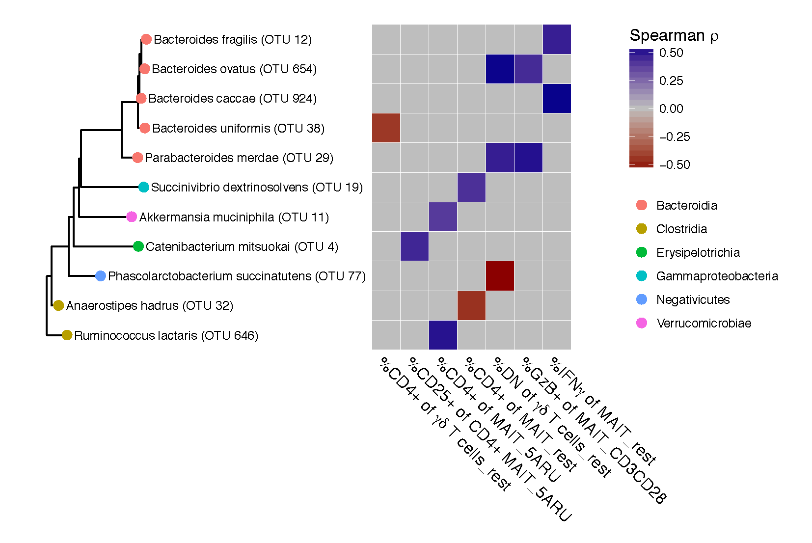
Below is the key output: cor_ht_dt_w$taxon are the taxa that correlate with immune phenotypes, and lefse.out$taxon are the taxa that are differentially abundant between Family Contacts and Community Controls. We intersect these and only look at taxa that are significant for both.

common <-intersect(lefse.out$taxon,cor_ht_dt_w$taxon)
phy_common <- prune_taxa(taxa = common,phy_contacts)

#Phylogenetic Tree
phy_sig<-prune_taxa(as.character(cor_ht_dt_w$taxon),phy_contacts)
p.species <- phy_common
library(yingtools2)
library(ggtree)
tr <- phy_tree(p.species)
spec <- as.data.frame(get.tax(p.species))
gt <- ggtree(tr, branch.length = "y",ladderize = T) %<+% spec
gd <- gt$data


data_eff <-  cor_ht_dt_w
rownames(data_eff) <-  cor_ht_dt_w$taxon
data_eff$taxon <-  NULL
data_eff <- as.matrix(data_eff)
#data_eff %>% View
g1 <- gt + geom_tippoint(aes(color=Order),size=3) + geom_tiplab(size =3)

# data_eff_cd4 <- data_eff[,1:8]
# data_eff_cd8 <- data_eff[,9:15]

g <- gheatmap(g1,data_eff,offset=2.5, width=2,colnames_angle=-45,hjust=0,font.size = 5) +
  scale_fill_gradient2(low = "darkred", mid = "grey",high = "darkblue")